Virtual sensors that know your process
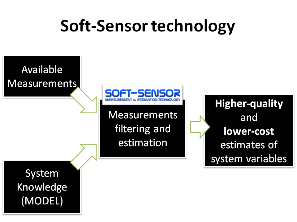
Soft-sensors combine system knowledge with available measurements to deliver reliable estimates of variables that are expensive, inaccessible, or impossible to measure directly.
What Are Soft-Sensors?
A soft-sensor — also called a virtual sensor — uses a mathematical model of the process together with existing measurement data to compute an estimate of a variable of interest. Unlike a physical instrument, a soft-sensor or virtual sensor requires no additional hardware — it runs as software on existing control systems, exploiting the instrumentation already in place.
Industry Problems Solved
Measurement is too expensive
Analytical instruments for quality, viscosity or composition cost €50k–€500k and are shared across streams — giving only periodic samples, not continuous data.
A soft-sensor delivers continuous estimates between analyzer samples, enabling tighter real-time control.
Instrumentation cannot be installed
Flow meters at valve locations, heat loads in cryogenic circuits, or torque in sealed drives cannot be instrumented due to cost, space, or harsh conditions.
A soft-sensor computes the variable from correlated upstream/downstream measurements already present in the system.
No direct measurement exists
Variables such as polymer melt index, cell concentration, or catalyst activity have no real-time in-line sensor technology.
A soft-sensor infers these variables from measurable proxies — temperature, pressure, flow, spectroscopy — using first-principles or data-driven models.
Sensor failure and redundancy
Critical measurements fail during startup, upset, or fouling. A single point of failure in a safety-critical loop cannot be tolerated.
A soft-sensor merges redundant measurements from multiple instruments or correlated variables to provide a fault-tolerant estimate that remains valid when individual sensors fail.
Measurement accuracy
Two instruments measuring the same variable may have complementary accuracy profiles — one fast but noisy, one slow but precise.
A soft-sensor fuses both signals using optimal estimation theory to produce an estimate that is simultaneously fast, precise, and drift-free.
Technology
Measurements
The exact sensor requirements are determined case by case. In most cases, existing instrumentation is sufficient — no new hardware is needed.
Models
Models encode the system knowledge exploited by the soft-sensor. Complexity ranges from simple empirical correlations to full thermo-hydraulic or kinetic dynamic models with hundreds of state variables. We specialise in first-principles modelling for process industry and aeronautical applications.
Estimation Algorithms
From linear observers (Luenberger, Kalman Filter) to nonlinear algorithms (Extended Kalman Filter, Unscented Kalman Filter, Moving Horizon Estimation). The choice depends on the degree of nonlinearity, available compute, and required accuracy.
Measured Results
- LHC cryogenic circuit (CERN): 5 thermodynamic states estimated in real time from 3 pressure sensors + temperature — nonlinear MHE at 1 Hz for superfluid helium below 2 K.
- Virtual flow meter at valve locations: continuous flow estimate without physical flow meter installation, reducing per-point instrumentation cost to software only.
- Sensor fusion variometer (SSDV12): pressure + IMU + GPS fusion delivering climb-rate resolution and accuracy beyond conventional barometric variometers.
- Analyzer gap coverage: continuous soft-sensor quality estimate between 2-hour laboratory sample intervals, enabling real-time quality control without additional analyzer investment.
Industrial Applications & Published Reference Results
Published benchmarks from peer-reviewed literature — what soft-sensor technology achieves in real industrial settings. Third-party results, each linked to its source.
Polymer melt index and density are only available from infrequent laboratory analysis (hours of delay). Quality control requires continuous real-time feedback across reactor temperature profiles and feed rates.
First-principles kinetic model inside NMPC closes the loop on delayed lab measurements, simultaneously controlling multiple reactors. Linear APC is insufficient due to strong nonlinear coupling between quality attributes and process conditions.
Basis weight (g/m²) cannot be measured in real time in the wire section of a tissue machine — only downstream, too late to correct production deviations.
Hybrid model: first-principles model (FPM) combined with 1D-CNN in parallel; a GRU network dynamically weights their outputs based on the current operating regime.
Permanent downhole gauges (PDGs) are expensive and unreliable in harsh well conditions. Bottom-hole pressure (BHP) is critical for production optimisation and flow assurance.
LSTM soft sensor trained on wellhead / topside measurements. Transfer Learning adapts the model across different well environments and operating conditions with minimal additional data.
Real-time NOx prediction is required for combustion optimisation and emissions compliance. Plant conditions shift continuously with load, fuel quality, and equipment ageing, causing static models to degrade quickly.
Just-In-Time Learning Random Forest (JIT-RF): adapts locally to current operating conditions at each prediction step, handling concept drift from combustion changes without full model retraining.
Lab analysis of effluent quality (COD, TSS, pathogen indicators) is slow and costly. No real-time visibility into treatment performance means delayed response to exceedances.
ML soft sensors trained on low-cost online measurements: turbidity, pH, conductivity. SVR (Support Vector Regression) and Cubist tree-based models predict key quality parameters continuously.
Tablet critical quality attributes (CQAs) — content uniformity, dissolution, hardness — are only measurable at end-of-batch, blocking Real-Time Release Testing (RTRT) and requiring full off-line QA.
Soft sensors infer CQAs from in-line PAT instruments (NIR, Raman, laser diffraction) and process data during manufacturing, following the FDA PAT guidance framework for science- and risk-based process understanding.
Metrology steps (CMP endpoint, film thickness, etch depth) are expensive and sampled at low frequency — creating quality blind spots across thousands of wafers between measurements.
Virtual Metrology (VM) predicts post-process quality from tool telemetry (RF power, chamber pressure, gas flows, process recipe) without physical measurement, enabling higher sampling density at near-zero cost.
Higher SAE automation levels require up to 28 sensors per vehicle at Level 5 vs 8 at Level 1. Physical sensors add cost, weight, power consumption, and failure points.
Virtual sensors (ideal, Hi-Fi, or RSI types) replace or supplement physical units, validated in full vehicle simulation environments. State estimation for chassis, drivetrain, and environment perception uses Kalman-family observers and hybrid ML approaches.
Soft Sensor / Virtual Sensor vs Physical Instrument
A direct comparison for procurement and feasibility decisions.
| Aspect | Physical Instrument | Soft Sensor / Virtual Sensor |
|---|---|---|
| Upfront cost | €50k–€500k per instrument | Software only — runs on existing DCS/PLC |
| Installation | Weeks to months (civil works, cabling) | Days to weeks (model integration) |
| Maintenance | Calibration shutdowns, fouling, replacement | Model update — no process downtime |
| Coverage | One physical location per device | Any variable reachable by the model |
| Data rate | Periodic (analyzer: 1–2 h) or single point | Continuous, synchronous with control cycle |
| Failure mode | Hard failure — loop goes open | Graceful degradation — model-only fallback |
Products
Advanced Virtual Flow Meter
Software-based flow calculation at valve locations using valve position, pressure and temperature measurements — no physical flow meter required.
Learn moreDigital Variometer SSDV12
High-precision climb/descent rate sensor for paraglider pilots using soft-sensor data fusion of pressure, inertial and GPS measurements.
Learn moreReferences
- Non-linear Moving Horizon State Estimation and Control for the Superfluid Helium Cryogenic Circuit at the Large Hadron Collider — IFAC, 2015. Dr. Noga contributed to this work during his PhD at CERN.
Selected Publications
Peer-reviewed research on soft-sensor and virtual sensor methods applied in industrial and scientific projects.
Frequently Asked Questions
What is a soft-sensor / virtual sensor?
A soft-sensor is a software model that computes estimates of hard-to-measure process variables from existing instrumentation. No new hardware is required — it runs on your existing DCS or PLC.
Do I need to install new sensors?
In most cases, no. The soft-sensor uses measurements already available in your control system. The exact requirements are assessed case by case.
How accurate are soft-sensors?
For well-instrumented processes with a good first-principles model, estimation errors of 1–5% are typical. The CERN LHC cryogenics application estimated 5 thermodynamic states from 3 pressure sensors.
How long does a project take?
Typically 4–12 weeks from kickoff to commissioning, depending on model complexity and data availability. A 30-minute feasibility call is enough to scope the work.
What happens when the process drifts or changes over time?
Process drift — from wear, feedstock variation, or production grade changes — is the most common cause of soft-sensor degradation. Robust deployments include model health monitoring (rolling RMSE, drift indicators), retraining triggers, and rollback to the previous model version. For processes with frequent regime changes, Just-In-Time (JIT) or adaptive models that recalibrate locally are preferred over static models.
Can a soft-sensor replace a physical sensor in a safety instrumented system?
Soft-sensors are highly valuable as advisory, monitoring, and redundant estimation channels. Using them as the sole measurement in a safety-critical loop (SIF) requires demonstrating deterministic failure modes, independence from other measurements, and full safety lifecycle compliance per IEC 61511. In practice, soft-sensors are deployed as a complement to physical safety instrumentation, not as a replacement for it.
Discuss Your Measurement Challenge
Every soft-sensor project starts with understanding your process, instrumentation, and what you need to measure. A 30-minute call is enough to assess feasibility.
About
Soft-Sensor is a specialised engineering practice led by Dr. Rafał Noga — APC/MPC consultant with experience in soft-sensor and state estimation for process industry, cryogenics, and aeronautics since 2007.